
前回、TesseractおよびPyTorchのニューラルネットワークで手書き数字の認識をやってみました。
今回は前回のPyTorchのニューラルネットワークに角度情報を加えて、手書き数字認識をやってみました。
具体的には、MNISTの28×28画像から、数字を線化処理し、8×8の2値画像に8段階の角度情報加えた8×8×8のデータで、512x1000x10の3層ニューラルネットワークを作り、自分の手書き数字をさせました。
結果、前回6~8割くらいだった正解率が9割くらいになりました。
追記:畳み込みニューラルネットワークもやってみたら更に高い正解率でした。
(ソースコードは記事の最後にあります)
環境:Windows10、Python3.8
プログラムの概要
ニューロンネットワークの構造は、入力層512個、中間層1000個、出力層10個です。
入力データは8×8の座標に対し、線の角度を8分割した8チャンネルとした8×8×8=512の一次行列で、線化された数字の線が8×8分割のある格子内にある時、その格子内の線の角度に応じたデータを1(プログラム上は255)とします。
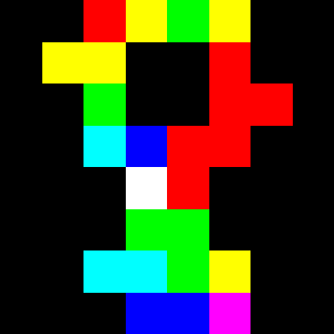
イメージとして分かりやすくするために、角度を3分割までにして、カラー表示させるとこんな感じ。
具体的な処理は、以下のような流れです。
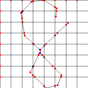
- 画像をスケルトン化および単純化(近似化)して、ポリラインデータ(点のリスト)に変換
- 線化した文字が95%くらいの大きさになるようにサイズおよび位置を調整
- 8×8の格子状の線データを作成し、ポリラインデータを格子と交差するところで線を分割
- 線毎に位置(どの格子内か)と角度を算出して、該当のデータに255を代入
細線化(スケルトン化)
細線化する処理をスケルトン化と呼ぶらしいです。Scikit-Imageという画像処理ライブラリにスケルトン化の機能があります。
Scikit-Imageでスケルトン化したラスタ画像をベクタ化するのに、Skeleton Network(sknw.py)というモジュールを使います。sknwにはnumba(高速化モジュール)を使用しているので、numbaもインストールします。
Scikit-Imageのインストール
pip install scikit-image
Skeleton Networkのインストール
他で使わないのであれば、sknw.pyを同フォルダにコピーするだけです。
Skeleton Network
https://github.com/Image-Py/sknw
Numbaのインストール
pip install numba
Python – ラスター画像からベクター画像への変換について
https://teratail.com/questions/244128
こんな感じの処理ができます(右はわざと単純化処理してます)
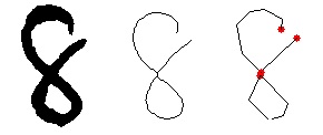
ちなみにOpenCVでも細線化の機能はあるのですが、ベクター化(ポリライン化)する方法がわからず、この方法を使いました。
データセットの作成
詰まると思っていたPyTorchの学習データセットの作成ですが、良質な記事のおかげか、そこまで詰まることなくできました。
pyTorchのtransforms,Datasets,Dataloaderの説明と自作Datasetの作成と使用
https://qiita.com/mathlive/items/2a512831878b8018db02
手書き数字の認識結果
まずはMNISTのtestingデータで正解率を測ってみます。
0:99.18 %
1:97.62 %
2:96.41 %
3:92.18 %
4:94.60 %
5:94.96 %
6:95.30 %
7:92.02 %
8:85.01 %
9:84.74 %
total: 93.24 %
全体の正解率は前回より落ちてしまいました。
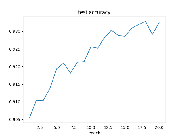
Accuracyはまだ上がり調子なので、学習回数が足りていないのかもしれません。
さて、自分の手書き数字は?
0( 90%): 0 0 0 6 0 0 0 0 0 0
1( 80%): 1 1 9 2 1 1 1 1 1 1
2(100%): 2 2 2 2 2 2 2 2 2 2
3( 90%): 3 3 3 3 3 3 3 3 3 2
4( 80%): 4 9 4 4 9 4 4 4 4 4
5(100%): 5 5 5 5 5 5 5 5 5 5
6(100%): 6 6 6 6 6 6 6 6 6 6
7(100%): 7 7 7 7 7 7 7 7 7 7
8(100%): 8 8 8 8 8 8 8 8 8 8
9( 80%): 7 9 9 9 9 9 9 9 7 9
total: 92.00 %
おお、NMISTのデータとほぼ変わらない正解率となりました。嬉しい!
文字サイズを80%に調整した画像データを使うと正解率97%。
0(100%): 0 0 0 0 0 0 0 0 0 0
1( 90%): 1 1 1 6 1 1 1 1 1 1
2(100%): 2 2 2 2 2 2 2 2 2 2
3( 90%): 3 3 3 3 3 3 3 3 3 7
4(100%): 4 4 4 4 4 4 4 4 4 4
5(100%): 5 5 5 5 5 5 5 5 5 5
6(100%): 6 6 6 6 6 6 6 6 6 6
7(100%): 7 7 7 7 7 7 7 7 7 7
8( 90%): 8 8 1 8 8 8 8 8 8 8
9(100%): 9 9 9 9 9 9 9 9 9 9
total: 97.00 %
まったく処理していない画像で正解率89%でした。
線化処理の過程で2値化や文字サイズ・位置の調整を行っているので、画像の前処理による差はでないはずっと思ってたんですけど、たまたま、ですかね。それでも、前回の時ほどデリケートではなく、9割くらいの正解率になっています。
正直、この正解率の向上が、角度情報が良かったのか、線化したことで線の太さのばらつきが軽減されたからなのか、数字の位置・サイズの調整を行ったからなのか、よく分かりません。
分かろうとするなら、色々なパターンを試す必要があるので、泥沼にはまりそうな気がします・・・。多分、ここから正解率95%くらいまでもっていくのも大変なんだろうなぁ。ということで、この辺でやめときます。
ソースは以下です。計算速度は全く考慮していません(せっかくnumpyの配列なのに普通にforループしてます)。
# -*- coding: utf-8 -*-
import os,random
import torch
import torchvision
import torch.nn.functional as f
from torch.utils.data import DataLoader
from torchvision import datasets, transforms
import matplotlib.pyplot as plt

import skeletonize

#NN info
im_width = 8
im_height = 8
im_channel = 8
im_datanum = im_width*im_height*im_channel

class MyNet(torch.nn.Module):
    def __init__(self):
        super(MyNet, self).__init__()
        self.fc1 = torch.nn.Linear(im_datanum, 1000)
        self.fc2 = torch.nn.Linear(1000, 10)

    def forward(self, x):
        x = self.fc1(x)
        x = torch.sigmoid(x)
        x = self.fc2(x)

        return f.log_softmax(x, dim=1)

class Mydatasets(torch.utils.data.Dataset):
    def __init__(self, data, labels, transform = None):
        self.transform = transform

        self.data = data
        self.label = labels

        self.datanum = len(self.label)
        print('datanum',self.datanum)

    def __len__(self):
        return self.datanum

    def __getitem__(self, idx):
        out_data = self.data[idx]
        out_label = self.label[idx]

        if self.transform:
            out_data = self.transform(out_data)

        return out_data, out_label

def training_mnist():
    # 学習回数
    epoch = 20

    batch = 100

    # 学習結果の保存用
    history = {
        'train_loss': [],
        'test_loss': [],
        'test_acc': [],
    }

    # ネットワークを構築
    net: torch.nn.Module = MyNet()

    # MNISTのデータローダーを取得
    train_loader = mnist_loader('S:/Temp/mnist_png/training',0,batch)
    test_loader = mnist_loader('S:/Temp/mnist_png/testing',0,batch)

    optimizer = torch.optim.Adam(params=net.parameters(), lr=0.001)

    for e in range(epoch):

        """ Training Part"""
        loss = None
        # 学習開始 (再開)
        net.train(True)
        for i, (data, target) in enumerate(train_loader):
            # 1次元化
            data = data.view(batch,im_datanum)

            optimizer.zero_grad()
            output = net(data)
            loss = f.nll_loss(output, target)
            loss.backward()
            optimizer.step()

            if i % 10 == 0:
                print('Training log: {} epoch ({} / 60000 train. data). Loss: {}'.format(e+1,
                                                                                         (i+1)*batch,
                                                                                         loss.item())
                      )

        history['train_loss'].append(loss)

        """ Test Part """
        # 学習のストップ
        net.eval()
        test_loss = 0
        correct = 0

        with torch.no_grad():
            for data, target in test_loader:
                data = data.view(-1,im_datanum)
                output = net(data)
                test_loss += f.nll_loss(output, target, reduction='sum').item()
                pred = output.argmax(dim=1, keepdim=True)
                correct += pred.eq(target.view_as(pred)).sum().item()

        test_loss /= 10000

        print('Test loss (avg): {}, Accuracy: {}'.format(test_loss,
                                                         correct / 10000))

        history['test_loss'].append(test_loss)
        history['test_acc'].append(correct / 10000)

    #モデルの保存
    torch.save(net.state_dict(), 'my_nn_model.pth')

    # 結果の出力と描画
    print(history)
    plt.figure()
    plt.plot(range(1, epoch+1), history['train_loss'], label='train_loss')
    plt.plot(range(1, epoch+1), history['test_loss'], label='test_loss')
    plt.xlabel('epoch')
    plt.legend()
    plt.savefig('loss.png')

    plt.figure()
    plt.plot(range(1, epoch+1), history['test_acc'])
    plt.title('test accuracy')
    plt.xlabel('epoch')
    plt.savefig('test_acc.png')


def mnist_loader(datapaths, sampling=0, batch=100):
    labels = []
    datalist = []
    for i in range(10):
        path = os.path.join(dirpath,str(i))
        flist = [f for f in os.listdir(path) if os.path.isfile(os.path.join(path,f))]
        if sampling:
            flist = random.sample(flist,sampling)
        datapaths = []
        for f in enumerate(flist):
            fp = os.path.join(path,f)

            data = skeletonize.create_data(fp,size=(im_width,im_height),
                                           channel=im_channel,invert=True)
            datalist.append(data)
            labels.append(i)
            if i % 100 == 0:
                print('creating data n='+str(len(labels)))

    trans = torchvision.transforms.ToTensor()
    dataset = Mydatasets(datalist,labels,trans)
    loader = torch.utils.data.DataLoader(dataset,batch,shuffle=True)

    return loader

def create_tensor(im_path,im_invert=False):
    data = skeletonize.create_data(im_path,invert=im_invert)
    transform=transforms.Compose([transforms.ToTensor()])
    data = transform(data)
    data = data.view(-1, im_datanum)
    return data

def prediction_single(im_path, im_invert=True):
    net: torch.nn.Module = MyNet()
    net.load_state_dict(torch.load('my_nn_model.pth'))
    net = net.eval()

    data = create_tensor(im_path,invert=invert)
    output = net(data)
    _, predict = torch.max(output, 1)

    print('result=' + str(predict[0].item()))

def test_prediction():

    net = MyNet()
    net.load_state_dict(torch.load('my_nn_model.pth'))
    net = net.eval()

    path = './img_src/'
    total_n = total_c = 0.0
    for i in range(10):
        files = os.listdir(path)
        flist = [f for f in files if os.path.isfile(os.path.join(path, f))]

        n = c = 0
        result = ''
        for j in range(10):
            f = str(i)+'-'+str(j)+'.png'
            filepath = os.path.join(path,f)
            data = create_tensor(filepath)
            output = net(data)
            _, prediction = torch.max(output, 1)
            # 結果を出力
            re = str(prediction[0].item())
            if str(i) == re:
                c += 1
            n += 1
            result += re+' '
        per = float(c)/float(n)*100
        total_c += c
        total_n += n
        print('%d(%d%%): %s' % (i,per,result))
    per = total_c/total_n*100
    print('total: %0.2f %%' % per)

def main():
    #training_mnist()
    test_prediction()

if __name__ == '__main__':
    main()
[skeletonize.py]
#!/usr/bin/env python
# -*- coding: utf-8 -*-
import os,math
import cv2
import numpy as np
from skimage.morphology import skeletonize
import sknw

def img_to_polylines(im_path,invert=True):

    img = cv2.imread(im_path)

    #2値化
    img = cv2.cvtColor(img, cv2.COLOR_BGR2GRAY)
    if invert:
        img = cv2.bitwise_not(img)
    img = cv2.GaussianBlur(img,(5,5),0)
    ret,img = cv2.threshold(img,0,255,cv2.THRESH_BINARY+cv2.THRESH_OTSU)

    #細線化(スケルトン化)
    ske = skeletonize(~(img != 0))
    ske_view = (ske * 255).astype(np.uint8)
    ske_view = cv2.cvtColor(ske_view, cv2.COLOR_GRAY2RGB)
    ske_view = cv2.bitwise_not(ske_view)
    graph = sknw.build_sknw(ske.astype(np.uint16), multi=True)

    #ポリラインの正規化
    xmin = ymin = float('inf')
    xmax = ymax = 0.0
    for (s,e) in graph.edges():
        for g in graph[s][e].values():
            for y,x in g['pts'].tolist():
                if x < xmin: xmin = x if x > xmax: xmax = x
                if y < ymin: ymin = y if y > ymax: ymax = y
    width = max(abs(xmax-xmin),abs(ymax-ymin))*1.05
    xshift = (width-(xmax-xmin))/2
    yshift = (width-(ymax-ymin))/2
    polylines = []
    for (s,e) in graph.edges():
        for g in graph[s][e].values():
            pts = []
            for y,x in g['pts'].tolist():
                x = float(x-xmin+xshift)/width
                y = float(y-ymin+yshift)/width
                pts.append((x,y))
            polylines.append(pts)
    #パスの簡略化
    new_polylines = []
    for pts in polylines:
        pts = np.array(pts, np.float32)
        epsilon = 0.02 #*cv2.arcLength(pts,False)
        approx = cv2.approxPolyDP(pts,epsilon,False)
        pts = []
        for pt in approx.tolist():
            pts.append(pt[0])
        new_polylines.append(pts)
    polylines = new_polylines

    return polylines

def split_lines(line,lattice_lines):
    split_lines = []
    split_lines.append(line)
    while True:
        has_crosspoint = False
        is_reset = False
        for line0 in split_lines:
            p0,p1 = line0
            for line1 in lattice_lines:
                p2,p3 = line1
                cp = cross_point(p0,p1,p2,p3)
                if not cp:
                    continue
                cp = cp[:2]
                d0 = distance(p0,cp)
                d1 = distance(p1,cp)
                if d0<0.000001 or d1<0.000001:
                    continue
                split_lines.remove(line0)
                split_lines.append((p0,cp))
                split_lines.append((cp,p1))
                has_crosspoint = True
                is_reset = True
                break
            if is_reset:
                break
        if not has_crosspoint:
            break
    return split_lines

def distance(p0,p1):
    d = (p1[0]-p0[0])**2+(p1[1]-p0[1])**2
    d = d**0.5
    return d

def cross_point(p0,p1,p2,p3):
    d = float((p1[0]-p0[0])*(p3[1]-p2[1])-(p1[1]-p0[1])*(p3[0]-p2[0]))
    if d == 0:
        return False
    ac = (p2[0]-p0[0],p2[1]-p0[1])
    t0 = ((p3[1]-p2[1])*ac[0] - (p3[0]-p2[0])*ac[1]) / d
    t1 = ((p1[1]-p0[1])*ac[0] - (p1[0]-p0[0])*ac[1]) / d
    if t0 < 0 or 1 < t0:
        return False
    if t1 < 0 or 1 < t1:
        return False
    x = p0[0] + t0*(p1[0] - p0[0])
    y = p0[1] + t0*(p1[1] - p0[1])
    p = [x,y]
    return p

def create_data(img_path,size=(8,8),channel=8,invert=False):
    #格子線作成
    lattice_lines = []
    for i in range(size[0]):
        x = i * 1.0 / size[0]
        line = ((x ,0.0),(x, 1.0))
        lattice_lines.append(line)
    for j in range(size[1]):
        y = j * 1.0 / size[1]
        line = ((0.0, y),((1.0),y))
        lattice_lines.append(line)

    #格子線で分割
    lines = []
    polylines = img_to_polylines(img_path,invert)
    for polyline in polylines:
        p0 = polyline.pop(0)
        for p1 in polyline:
            line = (p0,p1)
            lines += split_lines(line,lattice_lines)
            p0 = p1

    #位置、角度計算:データ作成
    data = np.zeros((size[1],size[0],channel),np.uint8)
    for line in lines:
        p0,p1 = line
        x = (p0[0]+p1[0])/2
        y = (p0[1]+p1[1])/2
        r = math.degrees(math.atan2(p1[1]-p0[1],p1[0]-p0[0]))
        if r < 0: r += 180
        r = r *0.99
        i = math.floor(x/(1.0/size[0]))
        j = math.floor(y/(1.0/size[1]))
        k = math.floor(r/(180.0/channel))
        data[j][i][k] = 255

    return data

    #for debug
    imsize = 300
    img = np.ones((imsize, imsize, 3))*255
    img = draw_lines(img,lines,imsize)
    img = draw_lines(img,lattice_lines,imsize)
    show(img)

    return data

def show_polylines(polylines):
    #線画の作成
    imsize = 100
    img = np.ones((imsize, imsize, 3))*255
    n = 1
    for pts in polylines:
        _p = pts.pop(0)
        x = int(_p[0]*imsize)
        y = int(_p[1]*imsize)
        img = cv2.circle(img,(x,y), 3, (0,0,255), -1)
        for p in pts:
            x0 = int(_p[0]*imsize)
            y0 = int(_p[1]*imsize)
            x1 = int(p[0]*imsize)
            y1 = int(p[1]*imsize)
            cv2.line(img,(x0,y0),(x1,y1),(0,0,0),1)
            _p = p
        n += 1
    show(img)

def draw_lines(img,lines,imsize = 100):
    n = 1
    for line in lines:
        p0,p1 = line
        x0 = int(p0[0]*imsize)
        y0 = int(p0[1]*imsize)
        x1 = int(p1[0]*imsize)
        y1 = int(p1[1]*imsize)

        img = cv2.line(img,(x0,y0),(x1,y1),(0,0,0),1)
        img = cv2.circle(img,(x0,y0), 3, (0,0,255), -1)
        img = cv2.circle(img,(x1,y1), 2, (255,0,0), -1)

    return img

def show(img):
    cv2.imshow('test',img)
    cv2.waitKey(0)
    cv2.destroyAllWindows()

def test_single_img(img_path,invert=True):
    data = create_data(img_path,(8,8),3,invert)
    img = cv2.resize(data,(300,300),interpolation=cv2.INTER_NEAREST)
    show(img)

def main():
    test_single_img('img2/7-0.png',invert=False)
    #test_single_img(r'S:\Temp\mnist_png\testing\1\1673.png')

if __name__ == '__main__':
    main()